How to use the NetworExtinction Package
Isidora Avila and Derek Corcoran
2020-11-09
#Introduction
The objectives of the NetworkExtinction package is to analyze and visualize the topology of food-webs and its responses to the simulated extinction of species.
The main indexes used for these analyzes are:
Number of nodes: Total number of species in the network (Dunne, Williams, and Martinez 2002).
Number of links: Number of trophic relationships represented in the food web (Dunne, Williams, and Martinez 2002).
Connectance: Proportion of all possible trophic links that are completed (Dunne, Williams, and Martinez 2002).
Primary removals: It occurs when the researcher intentionally removes one species, simulating a single extinction.
Secondary extinctions: A secondary extinction occurs when a non-basal species loses all of its prey items due to the removal of another species. In this context, basal species can experience primary removal, but not secondary extinctions (Dunne, Williams, and Martinez 2002).
Total extinctions: The sum of primary removal and secondary extinctions in one simulation.
This package was built with a total of six functions. There are four functions to analyze the cascading effect of extinctions in a food-web, one function to plot the results of any of the extinction analysis, and another to analize the degree distribution in the network.
Functions to analyze the cascading effect of extinctions are the following:
Mostconnected: To simulate extinctions from the most connected species to less connected in the network.
ExtinctionOrder: To simulate extinctions in a customized order.
RandomExtinctions: To develop a null hypothesis by generating random orders of simulated extinctions.
CompareExtinctions: To compare the observed secondary extinctions with the expected secondary extinction generated by random extinction.
The function to plot results is:
- ExtinctionPlot: To plot the results of any of the extinction functions
The function to analize the degree distribution is:
- degree_distribution: To test if the degrees in the network follow a power law, exponential, or truncated distribution.
0.1 How to install the package
As any package in cran the install.packages function can be used to intall de NetworkExtinction package as shown in the following code.
install.packages(NetworkExtinction)
library(NetworkExtinction)
0.2 How to represent a food-web in R
The first step to make any analysis in the NetworkExtinction package is to build a representation of a food-web, using the network package (Butts and others 2008).
In order to create a network object you can start with a matrix or an edgelist object (for more details see the network package vignette).
As an example of how to build a food-web we will explain how to create the network shown in figure 1.
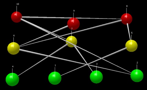
Figure 1. Food-web to be contructed in R
This network has ten nodes where each node represents one species. Here, four nodes are basal species (primary producers, from sp.1 to sp.4), three nodes are intermediate (primary consumers, from sp.5 to sp.7), and the remaining three are top predators (from sp.8 to sp.10).
In order to build an interaction matrix (Figure 2) that represent the food-web, we create a square matrix with a column and a row representing each species. Columns represent the consumers and the rows the resources, where 1 represents a trophic interaction and 0 its absence. Note that in the columns, the first four species only have zeros because they are not consumers. For example, if we look at species 7, it feeds on species 4 and 3. In order to represent that, we would go to column 7 and put a 1 in rows 3 and 4.
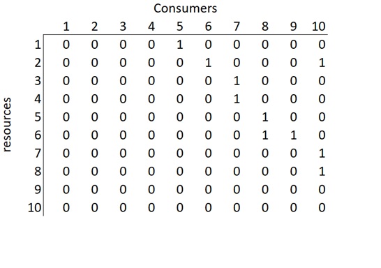
Figure 2. Matrix representation of the food-web
The following code is an example of how to build the matrix in figure 2 using R:
a<- matrix(c(0, 0, 0, 0, 0, 0, 0, 0, 0, 0, 0, 0, 0, 0, 0, 0, 0, 0, 0, 0, 0, 0, 0, 0, 0, 0, 0, 0, 0, 0, 0, 0, 0, 0, 0, 0, 0, 0, 0, 0, 1, 0, 0, 0, 0, 0, 0, 0, 0, 0, 0, 1, 0, 0, 0, 0, 0, 0, 0, 0, 0, 0, 1, 1, 0, 0, 0, 0, 0, 0, 0, 0, 0, 0, 1, 1, 0, 0, 0, 0, 0, 0, 0, 0, 0, 1, 0, 0, 0, 0, 0, 1, 0, 0, 0, 0, 1, 1, 0, 0),nrow=10, ncol=10)

a
#>       [,1] [,2] [,3] [,4] [,5] [,6] [,7] [,8] [,9] [,10]
#>  [1,]    0    0    0    0    1    0    0    0    0     0
#>  [2,]    0    0    0    0    0    1    0    0    0     1
#>  [3,]    0    0    0    0    0    0    1    0    0     0
#>  [4,]    0    0    0    0    0    0    1    0    0     0
#>  [5,]    0    0    0    0    0    0    0    1    0     0
#>  [6,]    0    0    0    0    0    0    0    1    1     0
#>  [7,]    0    0    0    0    0    0    0    0    0     1
#>  [8,]    0    0    0    0    0    0    0    0    0     1
#>  [9,]    0    0    0    0    0    0    0    0    0     0
#> [10,]    0    0    0    0    0    0    0    0    0     0
Once the matrix is ready, we use the as.network function from the network package to build a network object.
library(network)
net <- as.network(a, loops = TRUE)
net
#>  Network attributes:
#>   vertices = 10
#>   directed = TRUE
#>   hyper = FALSE
#>   loops = TRUE
#>   multiple = FALSE
#>   bipartite = FALSE
#>   total edges= 10
#>     missing edges= 0
#>     non-missing edges= 10
#>
#>  Vertex attribute names:
#>     vertex.names
#>
#> No edge attributes
1 Functions
1.1 Extinctions functions
1.1.1 Extinctions from most to less conected species in the network
The Mostconnected function sorts the species from the most connected node to the least connected node, using total degree. Then, it removes the most connected node in the network, simulating its extinction, and recalculates the topological indexes of the network and counts how many species have indegree 0 (secondary extinction), not considering primary producers. Then, it removes the nodes that were secondarily extinct in the previous step and recalculates which node is the new most connected species. This step is repeated until the number of links in the network is zero (Sole and Montoya 2001; Dunne, Williams, and Martinez 2002; Dunne and Williams 2009).
library(NetworkExtinction)
data("net")
Mostconnected(Network = net)
#> [1] 1
#> [1] 2
#> [1] 3
#> [1] 4| Spp | nodesS | linksS | Conectance | LinksPerSpecies | Secondary_extinctions | isolated_nodes | AccSecondaryExtinction | NumExt | TotalExt |
|---|---|---|---|---|---|---|---|---|---|
| 6 | 9 | 7 | 0.0864198 | 0.7777778 | 1 | 1 | 1 | 1 | 2 |
| 7 | 7 | 4 | 0.0816327 | 0.5714286 | 0 | 2 | 1 | 2 | 3 |
| 5 | 6 | 2 | 0.0555556 | 0.3333333 | 1 | 3 | 2 | 3 | 5 |
| 2 | 4 | 0 | 0.0000000 | 0.0000000 | 1 | 4 | 3 | 4 | 7 |
The result of this function is the dataframe shown in table 1. The first column called Spp indicates the order in which the species were removed simulating an extinction. The column Secondary_extinctions represents the numbers of species that become extinct given that they do not have any food items left in the food-web, while the AccSecondaryExtinction column represents the accumulated secondary extinctions. (To plot the results, see function ExtinctionPlot.)
data("net")
history <- Mostconnected(Network = net)
#> [1] 1
#> [1] 2
#> [1] 3
#> [1] 4
ExtinctionPlot(History = history, Variable = "AccSecondaryExtinction")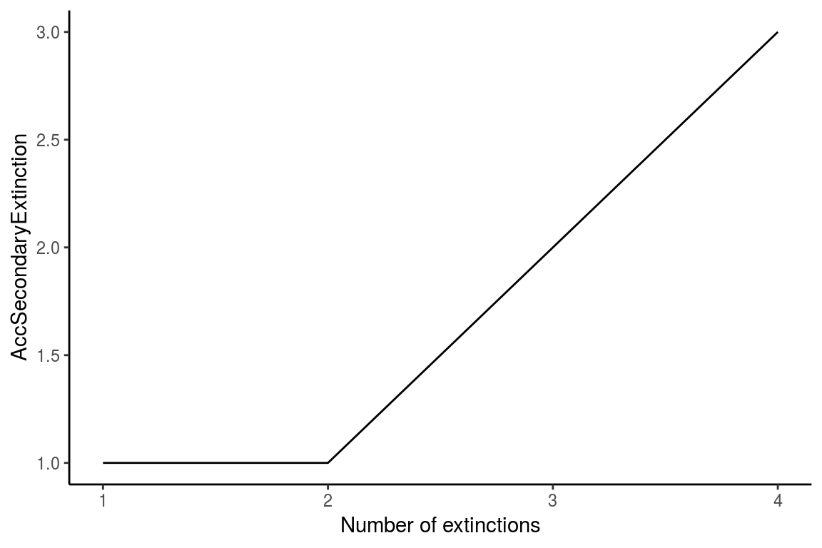
Figure 3. The graph shows the number of accumulated secondary extinctions that occur when removing species from the most to the least connected species
1.1.2 Extinctions using a customized order
The ExtinctionOrder function takes a network and extinguishes nodes using a customized order. Then, it calculates the topological network indexes and the secondary extinctions.
data("net")
ExtinctionOrder(Network = net, Order = c(2,4,7))| Spp | nodesS | linksS | Conectance | Secondary_extinctions | AccSecondaryExtinction | NumExt | TotalExt |
|---|---|---|---|---|---|---|---|
| 2 | 9 | 8 | 0.0987654 | 1 | 1 | 1 | 2 |
| 4 | 7 | 5 | 0.1020408 | 1 | 2 | 2 | 4 |
| 7 | 5 | 3 | 0.1200000 | 0 | 2 | 3 | 5 |
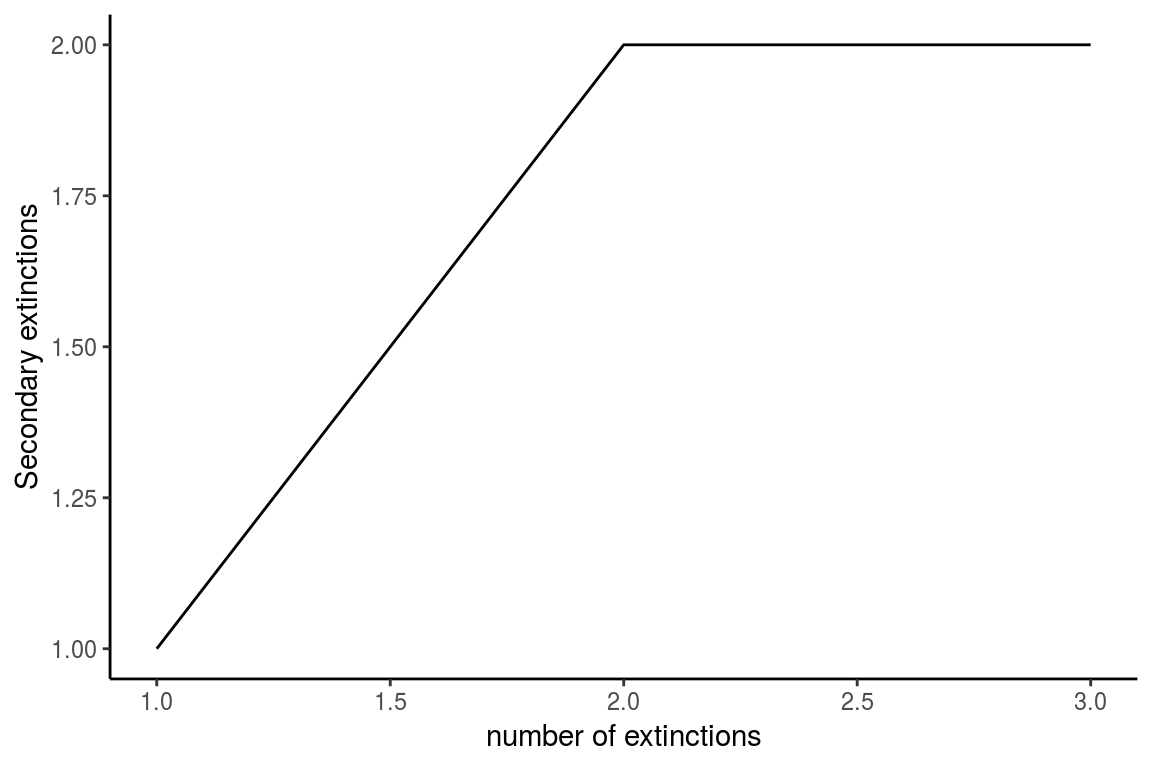
Figure 4. The graph shows the number of accumulated secondary extinctions that occur when removing species in a custom order. In this example species 2 is removed followed by 4 and lastly species 7 is removed
The results of this function are a dataframe with the topological indexes of the network calculated from each extinction step (Table 2), and a plot that shows the number of accumulated secondary extinctions that occured with each removed node (Figure 4).
1.1.3 Random extinction
The RandomExtinctions function generates n random extinction orders, determined by the argument nsim. The first result of this function is a dataframe (table 3). The column NumExt represents the number of species removed, AccSecondaryExtinction is the average number of secondary extinctions for each species removed, and SdAccSecondaryExtinction is its standard deviation. The second result is a graph (figure 5), where the x axis is the number of species removed and the y axis is the number of accumulated secondary extinctions. The solid line is the average number of secondary extinctions for every simulated primary extinction, and the red area represents the mean \(\pm\) the standard deviation of the simulations.
data(net)
RandomExtinctions(Network= net, nsim= 500)| NumExt | SdAccSecondaryExtinction | AccSecondaryExtinction |
|---|---|---|
| 1 | 0.4587165 | 0.300000 |
| 2 | 0.7549941 | 0.682000 |
| 3 | 0.9540547 | 1.140000 |
| 4 | 1.0935849 | 1.592000 |
| 5 | 1.1795574 | 1.993865 |
| 6 | 1.2518519 | 2.235981 |
| 7 | 1.1971914 | 2.231270 |
| 8 | 1.1779286 | 2.258065 |
| 9 | 1.1227299 | 2.320755 |
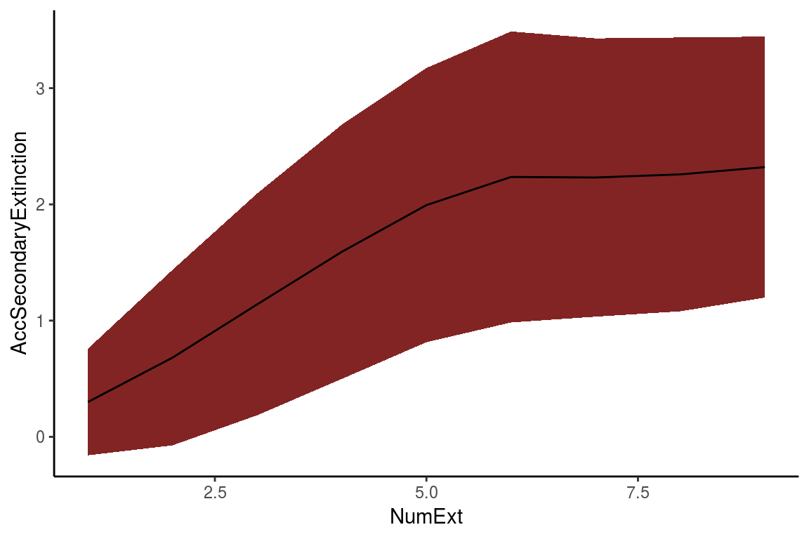
Figure 5. The resulting graph of the RandomExtinctions function
###Comparison of Null hypothesis with other extinction histories
The RandomExtinctons function generates a null hypothesis for us to compare it with either an extinction history generated by the ExtinctionOrder function or the Mostconnected function. In order to compare the expected extinctions developed by our null hypothesis with the observed extinction history, we developed the CompareExtinctions function. The way to use this last function is to first create the extinction history and the null hypothesis, and then the CompareExtinctins function to compare both extinction histories.
data("net")
History <- ExtinctionOrder(Network = net, Order = c(1,2,3,4,5,6,7,8,9,10))

set.seed(2)
NullHyp <- RandomExtinctions(Network = net, nsim = 500)

Comparison <- CompareExtinctions(Nullmodel = NullHyp, Hypothesis = History)
The first result will be a graph (Figue 6) with a dashed line showing the observed extinction history and a solid line showing the expected value of secondary extinctions randomly generated.
The second result will be a Test object which will show the goodness of fit statistics of the comparison. In this case, since the p value is 0.22 which is larger than 0.05, we consider that the generated extinction history is significantly different than the null hypothesis.
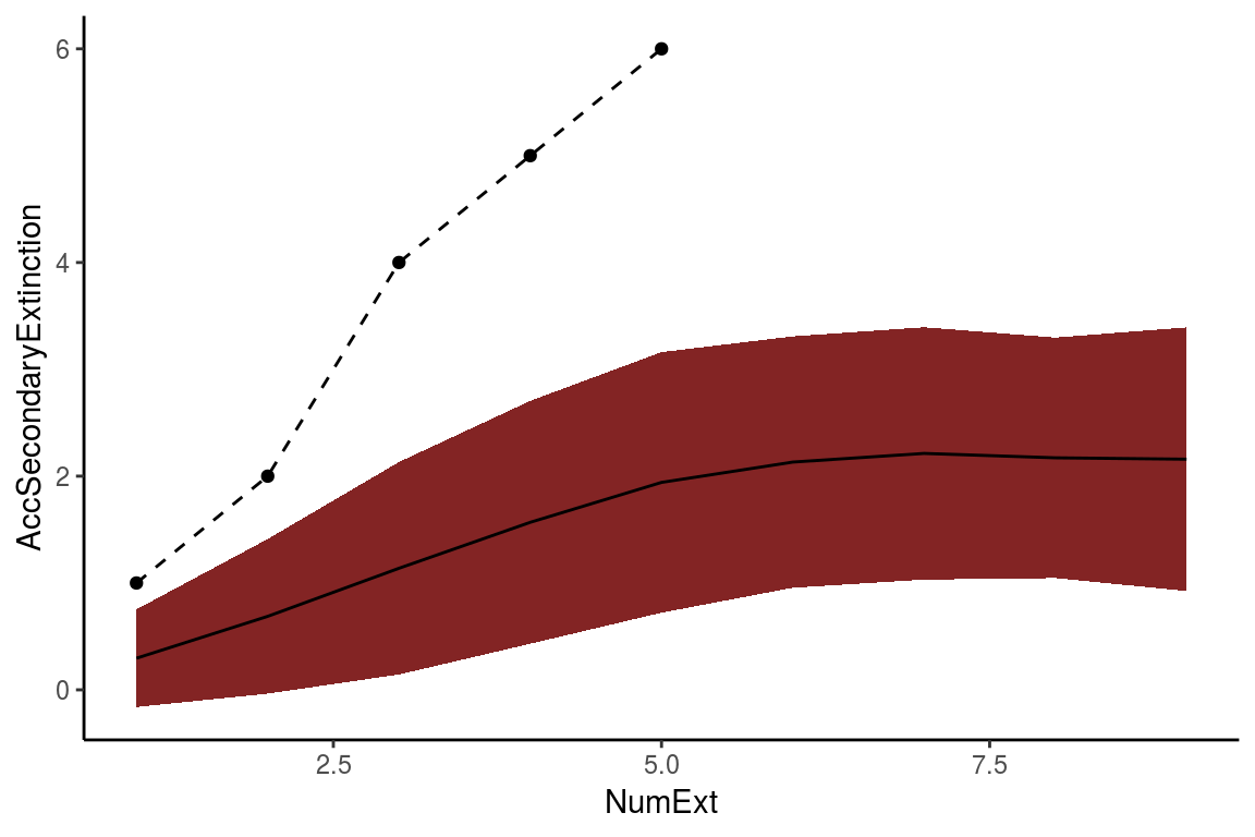
Figure 6. The resulting graph of the CompareExtinctions function, where the dashed line shows the observed extinction history, and a solid line shows the expected value of secondary extinctions originated at random
Comparison$Test
#>
#>  Pearson's Chi-squared test
#>
#> data:  Hypothesis$DF$AccSecondaryExtinction and Nullmodel$sims$AccSecondaryExtinction[1:length(Hypothesis$DF$AccSecondaryExtinction)]
#> X-squared = 20, df = 16, p-value = 0.2202
1.2 Plotting the extinction histories of a network
The ExtinctionPlot function takes a NetworkTopology class object and plots the index of interest after every extinction. By default, the function plots the number of accumulated secondary extinctions after every primary extinction (Figure 7), but any of the indexes can be ploted with the function by changing the Variable argument (Figure 8).
data(net)
history <- Mostconnected(Network = net)
#> [1] 1
#> [1] 2
#> [1] 3
#> [1] 4
ExtinctionPlot(History = history)
Figure 7. Example of the use of the ExtinctionPlot function showing the accumulated secondary extinctions against number of extinctions
ExtinctionPlot(History = history, Variable = "LinksPerSpecies")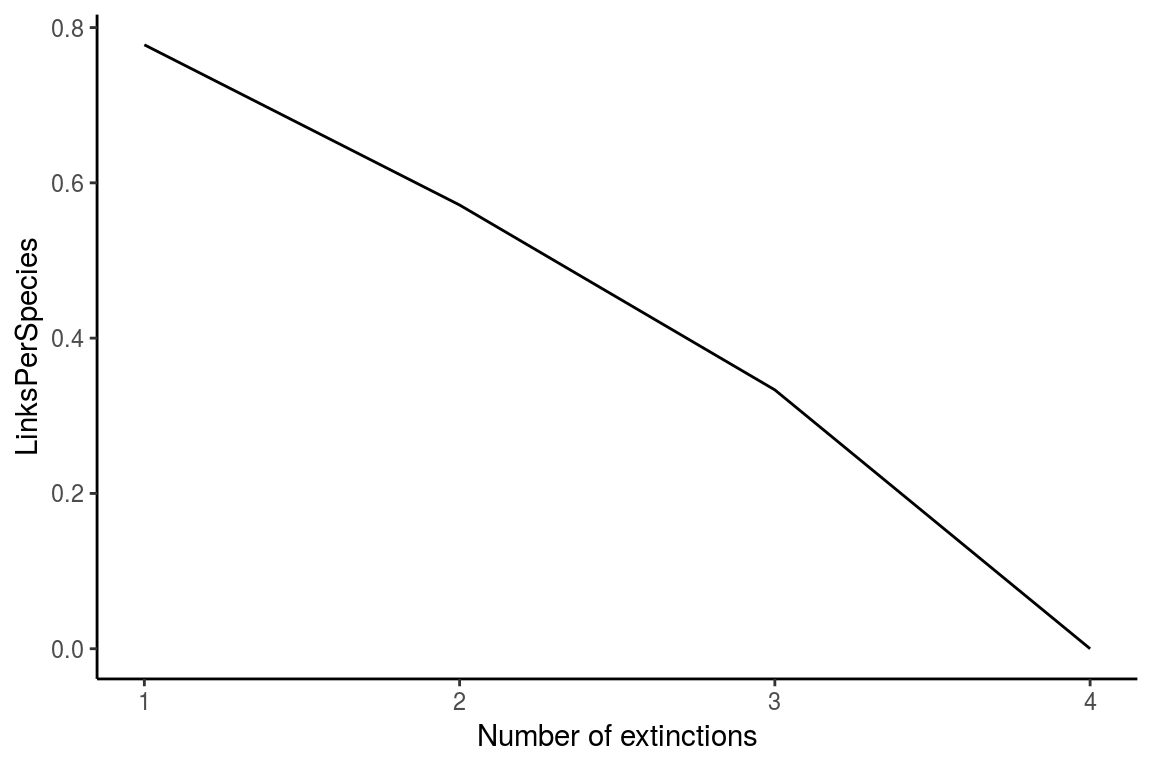
Figure 8. Another example of the use of the ExtinctionPlot function showing the number of links per species against number of extinctions
1.3 Degree distribution function
The degree_distribution function calculates the cumulative distribution of the number of links that each species in the food network has (Estrada 2007). Then, the observed distribution is fitted to the exponential, power-law and truncated power-law distribution models.
The results of this function are shown in figure 9 and table 4. The graph shows the observed degree distribution in a log-log scale fitting the three models mentioned above, for this example we use an example dataset of Chilean litoral rocky shores (Kéfi et al. 2015). The table shows the fitted model information ordered by descending AIC, that is, the model in the first row is the most probable distribution, followed by the second an finally the third distribution in this case (Table 3), the Exponential distribution would be the best model, followed by the Power-law and finally the Truncated power-law model.
data("chilean_intertidal")
degree_distribution(chilean_intertidal, name = "Test")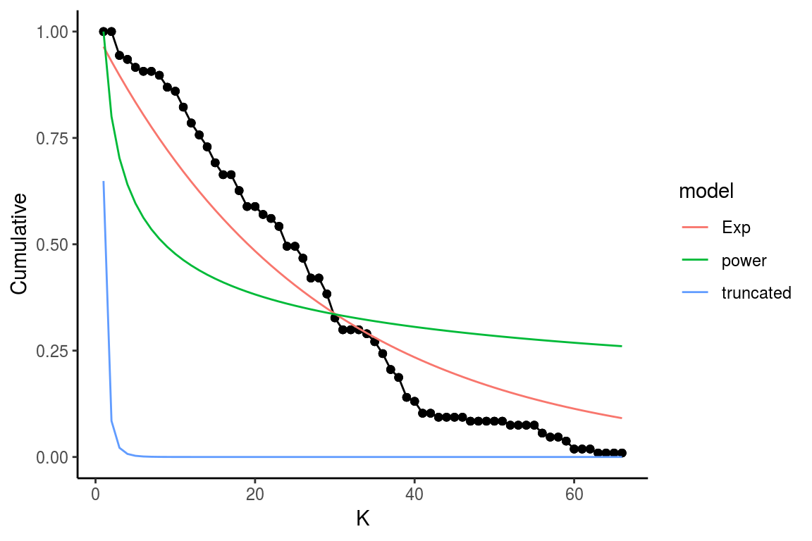
Figure 9: Fitted vs observed values of the degree distribution. The black line and points show the observed values, the red, green and blue lines show the fitted values for the Exponential, power law and trucated distribution, respectively
| sigma | isConv | finTol | logLik | AIC | BIC | deviance | df.residual | model |
|---|---|---|---|---|---|---|---|---|
| 0.0922763 | TRUE | 8.8e-06 | 66.057711 | -128.115423 | -123.676408 | 0.5704994 | 67 | Exponential |
| 0.2246009 | TRUE | 2.3e-06 | 5.420293 | -6.840586 | -2.461276 | 3.2789603 | 65 | Power |
| 0.4845141 | TRUE | 3.2e-06 | -45.321942 | 94.643884 | 99.023194 | 15.2590056 | 65 | truncated |
The main objective of fitting the cumulative distribution of the degrees to those models, is to determine if the vulnerability of the network to the removal of the most connected species is related to their degree distribution. Networks that follow a power law distribution are very vulnerable to the removal of the most connected nodes, while networks that follow exponential degree distribution are less vulnerable to the removal of the most connected nodes (see Albert and Barabási 2002, @dunne2002food, @estrada2007food, @de2013topological).
#Bibliography
Albert, Réka, and Albert-László Barabási. 2002. “Statistical Mechanics of Complex Networks.” Reviews of Modern Physics 74 (1). APS: 47.
Butts, Carter T, and others. 2008. “Network: A Package for Managing Relational Data in R.” Journal of Statistical Software 24 (2): 1–36.
Dunne, Jennifer A, and Richard J Williams. 2009. “Cascading Extinctions and Community Collapse in Model Food Webs.” Philosophical Transactions of the Royal Society B: Biological Sciences 364 (1524). The Royal Society: 1711–23.
Dunne, Jennifer A, Richard J Williams, and Neo D Martinez. 2002. “Food-Web Structure and Network Theory: The Role of Connectance and Size.” Proceedings of the National Academy of Sciences 99 (20). National Acad Sciences: 12917–22.
Estrada, Ernesto. 2007. “Food Webs Robustness to Biodiversity Loss: The Roles of Connectance, Expansibility and Degree Distribution.” Journal of Theoretical Biology 244 (2). Elsevier: 296–307.
Kéfi, Sonia, Eric L Berlow, Evie A Wieters, Lucas N Joppa, Spencer A Wood, Ulrich Brose, and Sergio A Navarrete. 2015. “Network Structure Beyond Food Webs: Mapping Non-Trophic and Trophic Interactions on Chilean Rocky Shores.” Ecology 96 (1). Wiley Online Library: 291–303.
Santana, Charles N de, Alejandro F Rozenfeld, Pablo A Marquet, and Carlos M Duarte. 2013. “Topological Properties of Polar Food Webs.” Marine Ecology Progress Series 474: 15–26.
Sole, Ricard V, and M Montoya. 2001. “Complexity and Fragility in Ecological Networks.” Proceedings of the Royal Society of London B: Biological Sciences 268 (1480). The Royal Society: 2039–45.
Copyright © 2017 Cienciaustral, Inc. ![]() All rights reserved.
All rights reserved.