Starting to use the Spatialball2 package
Derek Corcoran, and Nicholas Watanabe
2020-11-09
#Introduction
The SpatialBall2 package was developed to analyze and visualize spatial data in the NBA. We can separate the Spatialball functions into three groups:
- Data scraping
- Data visualization
- Data analysis
library(SpatialBall2)0.1 Data scraping
The Seasonscrape function, downloads data from the NBA.stats.com site the information needed for all the visualizations and analyses made in this package. You can request different seasons, and limit it to a range of dates, select if you want to analyse Regular season, playoffs, preseason, etc.
As an example on how to scrape data from the 2017-18 for a given date is shown bellow.
SeasonData2018 <- Seasonscrape(season = "2017-18", Start = "12/05/2017", End = "12/07/2017")The only parameter that is mandatory for this function is season. If you only fill that parameter, you will get all the data from the regular season of the year you requested.
0.2 Data visualization
We have three levels of data visualization with graphs at the player, team, and league level. We will go into detail in each of those categories. First for players and all other levels of visualization we have shot charts. In our shot charts (see Fig. 1 as an example) the color scheme will be a scale of the points per shot or percentage depending on the options you choose. The size of the hexagon in shot charts represents the frequency of the shots taken, by the league, team or player, with bigger hexagons meaning a higher frequency of shots. Now we will go in detail into each of the visualizations available in our package.
0.2.1 Player level visualization
0.2.1.1 Player shot charts
For any given player that played in the league on a given season, you can build shot charts. The main function to do that is ShotSeasonGraphPlayer, in its most basic configuration, you only need to use the parameters Seasondata and the name of the player, as seen in figure 1.
data("season2017")
ShotSeasonGraphPlayer(season2017, player = "Stephen Curry")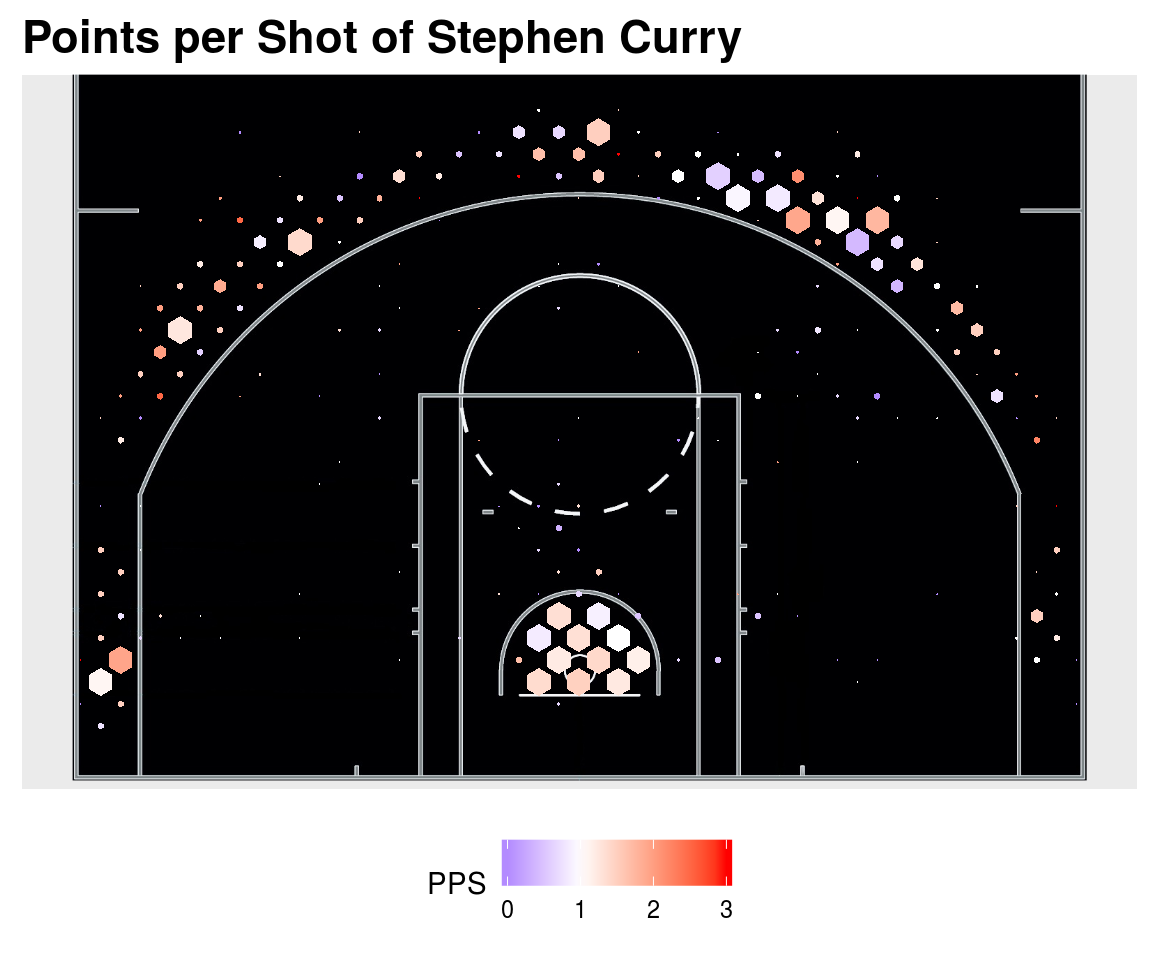
Figure 1. Shot chart of Stephen Curry
If you change the type parameter from “PPS” (Points Per Shot), which is the default, to “PCT” (Percentage of shots made), the color scale of the hexagon will change to reflect that, as seen in figure 2.
ShotSeasonGraphPlayer(season2017, player = "Stephen Curry", type = "PCT")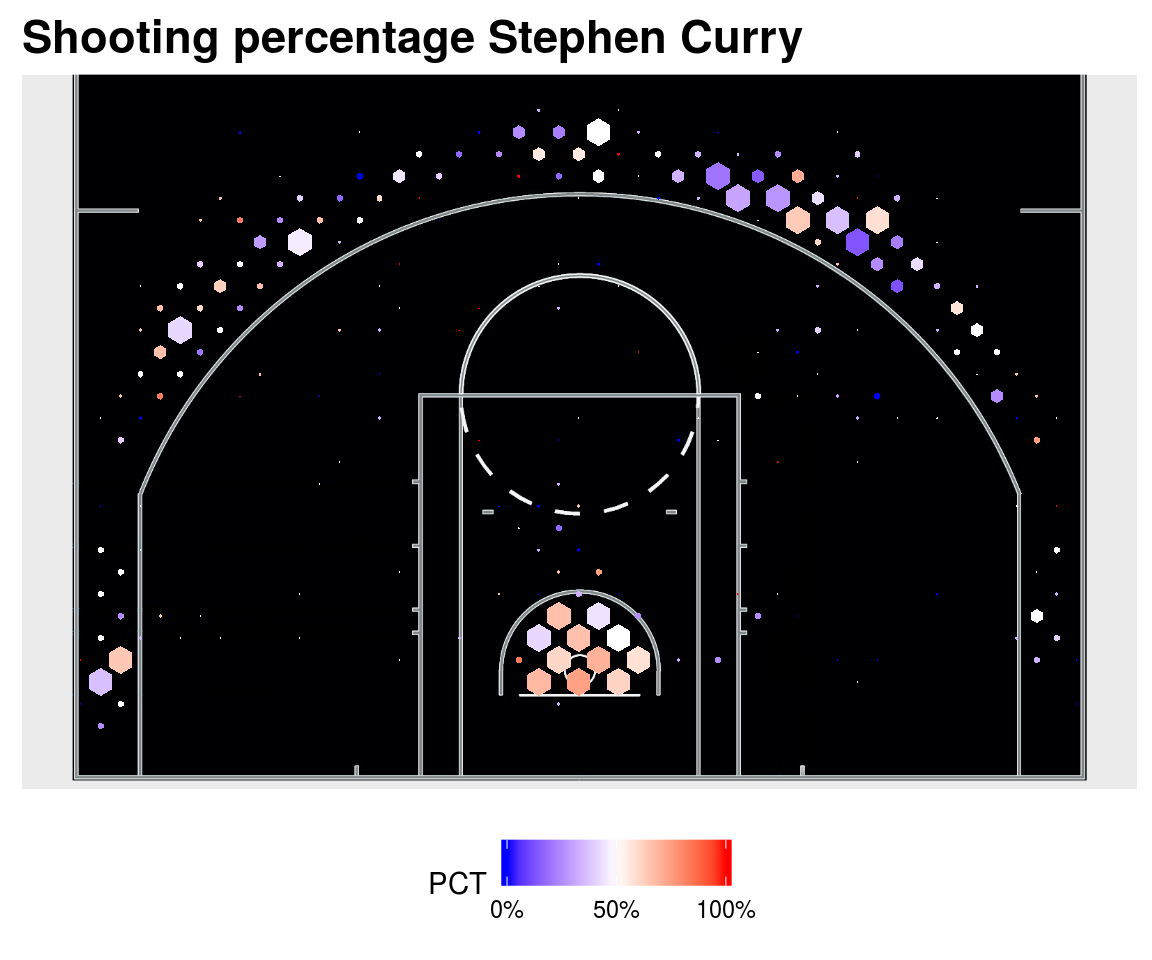
Figure 2. Shot chart of Stephen Curry showing the percentage of shots made
0.2.1.2 Player point shot charts
When it’s early in the season, or a player does not shot to much, making a frequency based shot chart might not be the best visualization tool. For that, we created the PointShotSeasonGraphPlayer. This function creates a shot chart for a player on a given season plotting a point for each taken shot separating by colors made and misses, Also, you can add a kernel of the frequency of usage of areas. For example here is the “traditional” shot chart of Kyle Singler (Figure 3).
data("season2017")
ShotSeasonGraphPlayer(season2017, player = "Kyle Singler")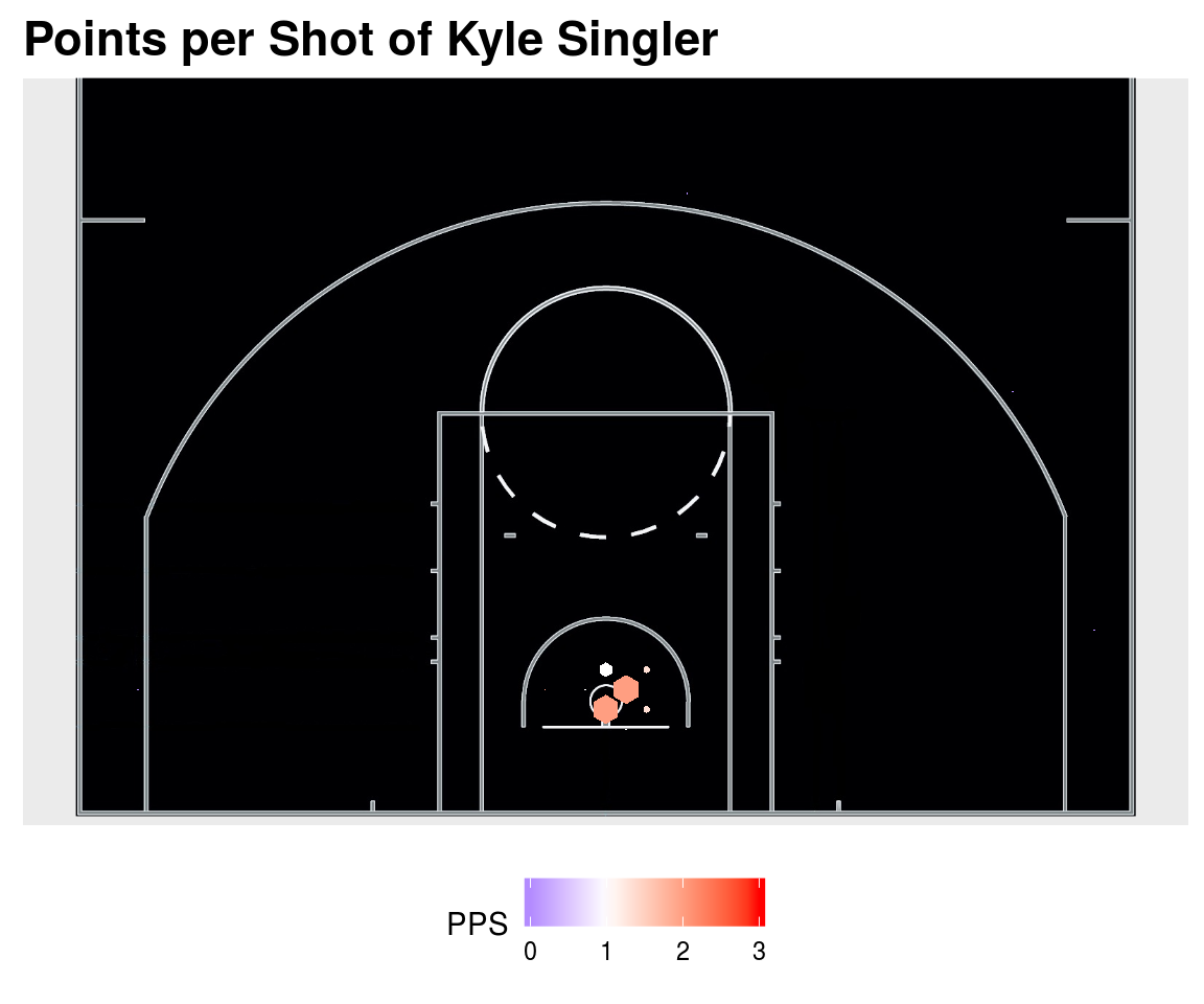
Figure 3. Shot chart of Kyle Singler
He only took 83 shots during the 2016-17 season, in that case, it might be better to plot every shot and a kernel of the most active areas for that player (Figure 4)
PointShotSeasonGraphPlayer(season2017, player = "Kyle Singler")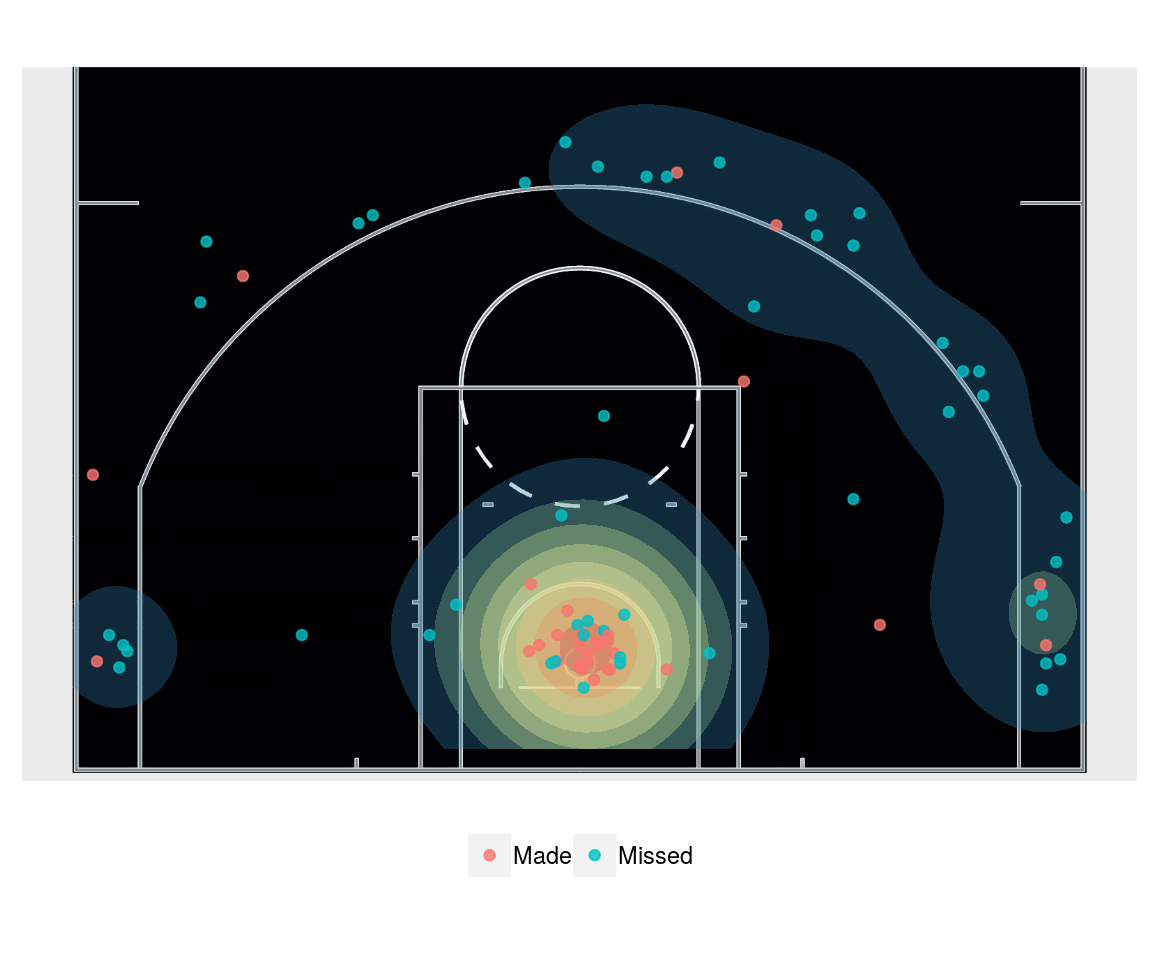
Figure 4. Shot chart of Kyle Singler, point and kernel
We can show only the made shots as shown in figure 5, and/or remove the kernel as shown in figure 6.
PointShotSeasonGraphPlayer(season2017, player = "Kyle Singler", Type = "Made")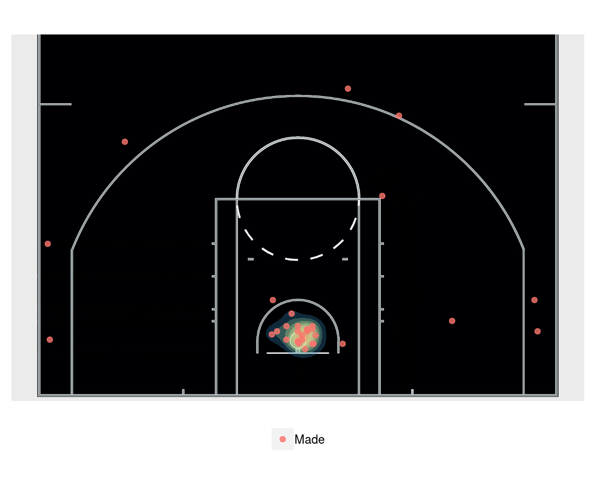
Figure 5. Shot chart of Kyle Singler, point and kernel, only made shots
PointShotSeasonGraphPlayer(season2017, player = "Kyle Singler", Type = "Made", kernel = FALSE)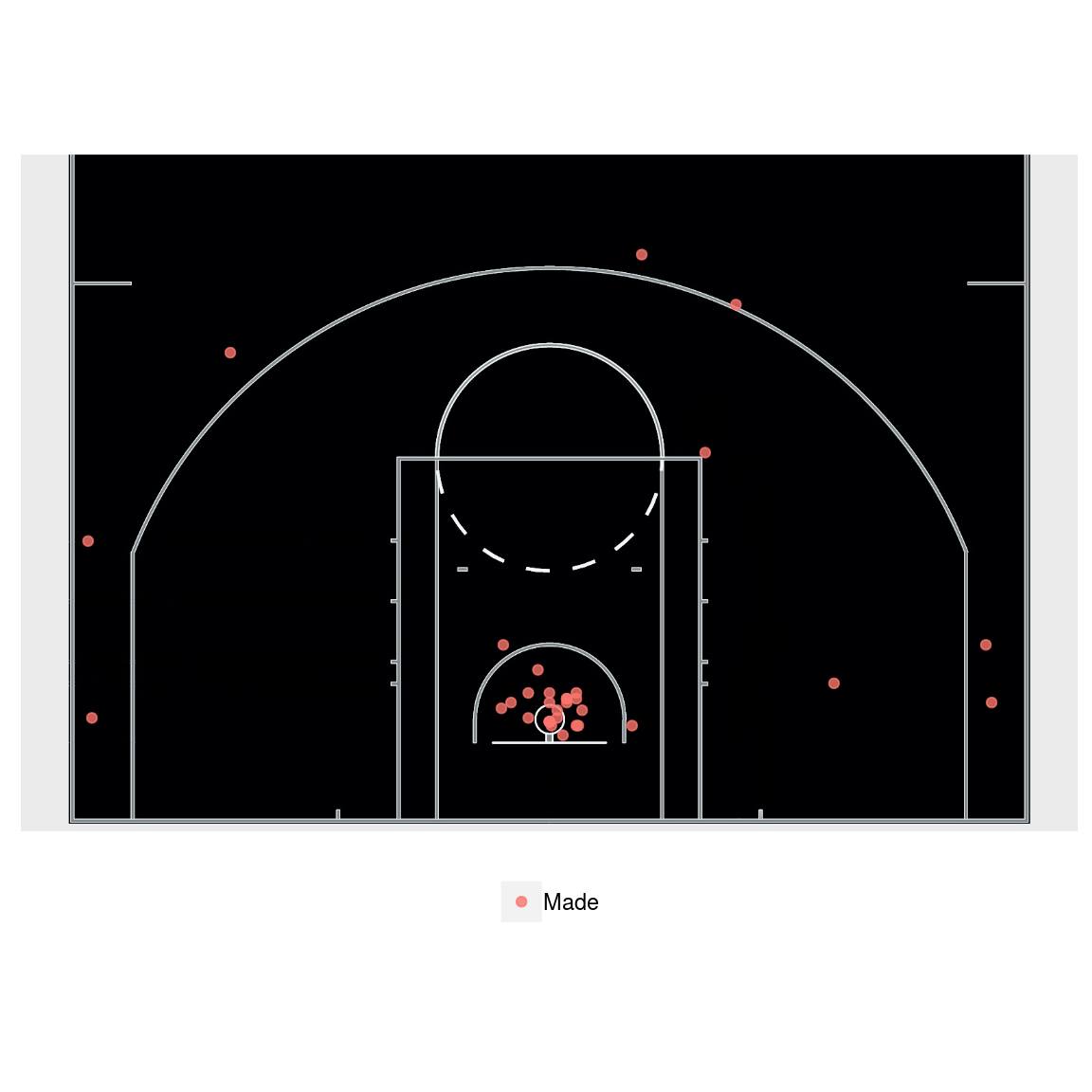
Figure 6. Shot chart of Kyle Singler, points only, only made shots
0.2.2 Team level visualization
0.2.2.1 Offensive shot charts
This shot charts are made from the shots that the selected team has taken. The function to make team offensive shotcharts is OffShotSeasonGraphTeam, where in the most basic option for this function, you only have to provide the Seasondata and the team parameters. As an example of these, lets plot the offensive shot chart of the Golden State Warriors from the 2016-17 season with the data included in the package.
OffShotSeasonGraphTeam(season2017, team = "GSW")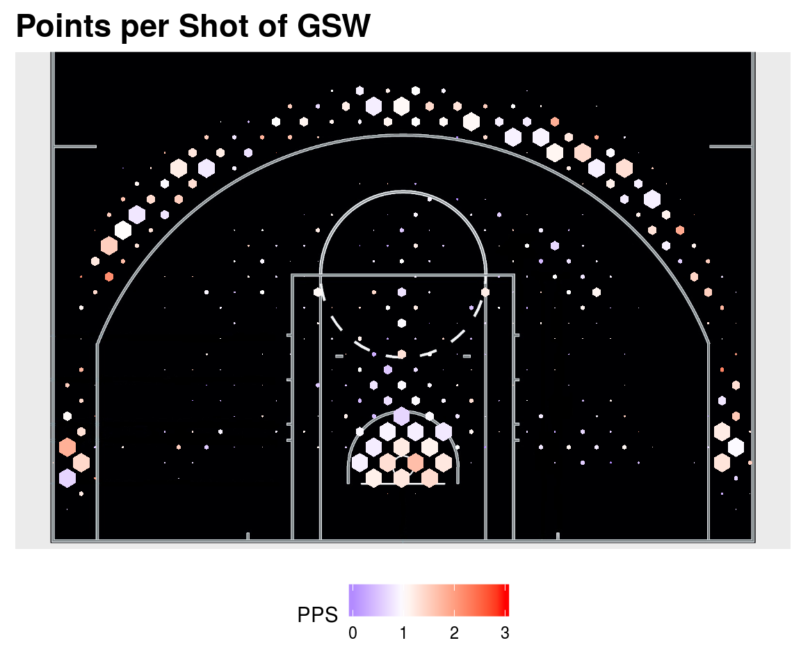
Figure 7. Offensive Shot chart of the Golden State Warriors
A we saw, the default graph has a color legend that varies according to the points per shot (PPS) of the team. This can be changed by changing the type parameter from "PPS" to "PCT" as follows.
data("season2017")
OffShotSeasonGraphTeam(season2017, team = "GSW", type = "PCT")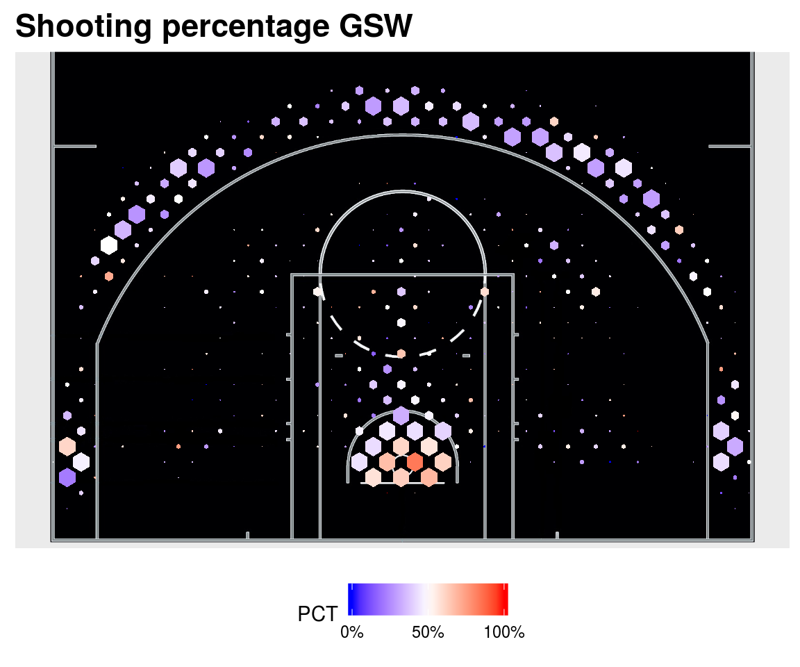
Figure 8. Offensive Shot chart of the Golden State Warriors, percentage of shots made
0.2.2.2 Defensive shot charts
Similar to the offensive shot charts, here we visualize the Points per shot or percentage allowed by the team we choose to graph, using the function DefShotSeasonGraphTeam. Similar to the functions OffShotSeasonGraphTeam and ShotSeasonGraphPlayer, this function allows the user to choose to visualize the shot chart with a Points per Shot or Percentage scale as seen in figure 8.
data("season2017")
DefShotSeasonGraphTeam(season2017, team = "Sas", type = "PCT")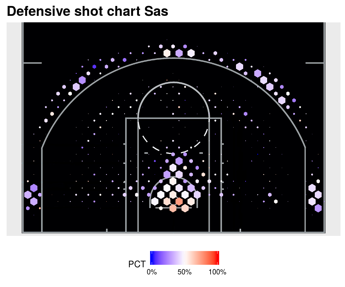
Figure 9. Offensive Shot chart of the Golden State Warriors, percentage of shots made
0.2.2.3 Comparative shot charts
The function to visually compare two teams it’s called ShotComparisonGraph, and it uses our comparative shot charts, in this example we have Miami against Houston. In the top row we see the defensive shot chart of the Heat, the Offensive Shot Chart of the rockets, and the net Shot Chart of the expected points per Shot over average when Rockets offense faces the Heat Defense. This plot takes into account both the shot frequency attempted by the offense and defense and assumes that the shot frequency for each area in the court will be an in-between frequency. At points where the hexagons are blue, the defense is allowing fewer points than average and the offense is scoring fewer points than average, and the inverse is true for red hexagons. Conversely the bottom row shows what happens when the Heat attacks and the Rockets defend.
ShotComparisonGraph(HomeTeam = "Hou", VisitorTeam = "Mia", Seasondata = season2017)
Figure 10. Comparative shot chart of 2016-17 Miami Heat against Houston Rockets
We can focus on the areas where the offensive team is favored by adding to the code the focus = “plus” command, as follows, which will change only the last column of the graph.
ShotComparisonGraph(HomeTeam = "Hou", VisitorTeam = "Mia", Seasondata = season2017, focus = "plus")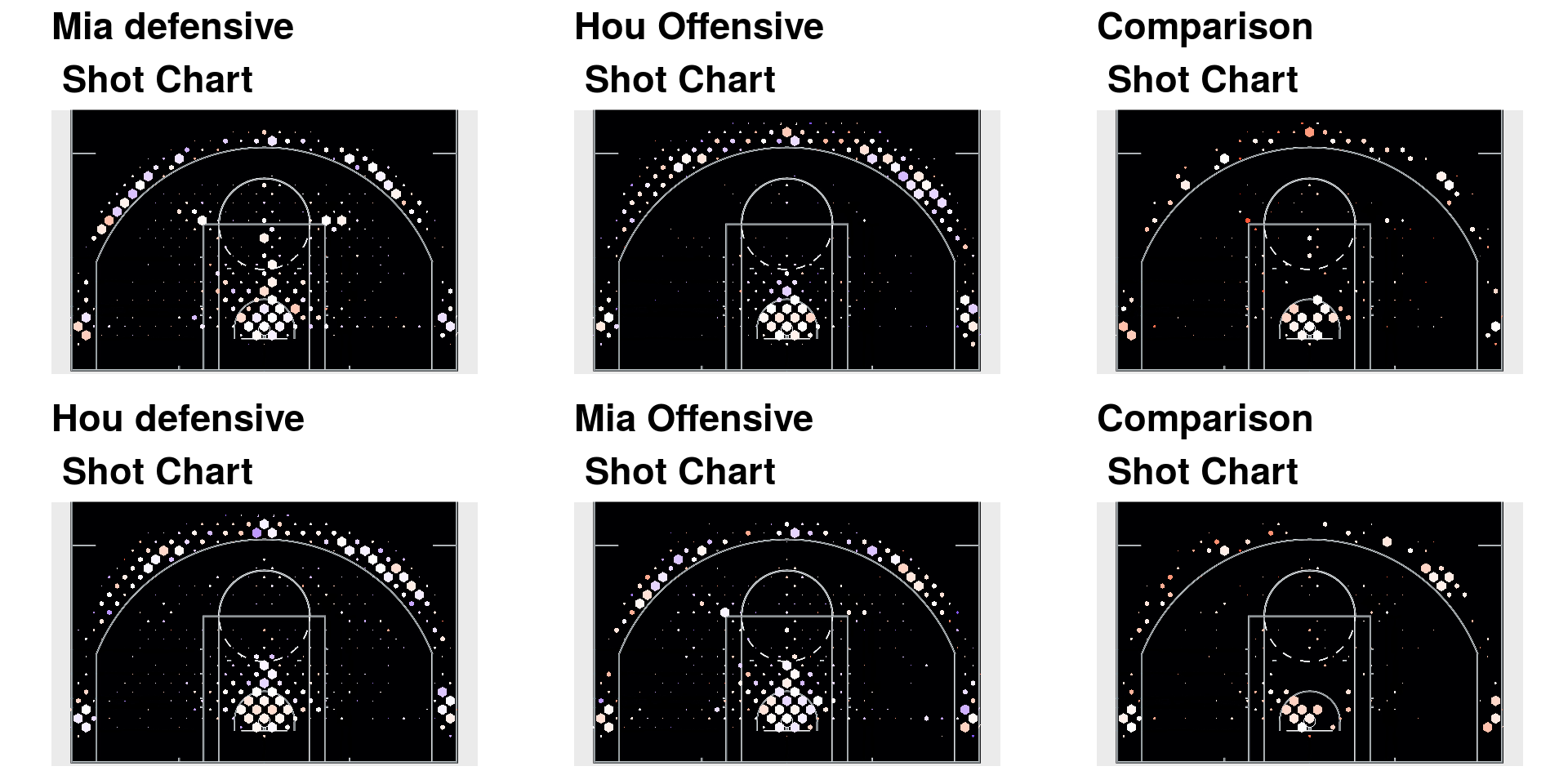
Figure 11. Comparative shot chart of 2016-17 Miami Heat against Houston Rockets, focusing in the areas where the attack has the advantage
0.2.3 League level visualization
The ShotSeasonGraph function takes an NBA season object and makes a shot chart of all the shots takes through that regular season. You can choose to either plot the results based on Points per Shot or on Shooting Percentage, as in all previous functions. This function is exemplified in figure 12.
data("season2017")
ShotSeasonGraph(season2017, quant = 0.4)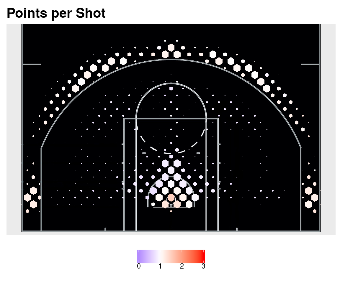
Figure 12. Shot chart of the Whole 2017 Season
0.3 Data analysis
###Offensive and defensive team stats
The TeamStats function are the basis of the table shown in this link which is updated daily. The only parameter needed for this function is the Seasondata parameter, which can be extracted from the Seasonscrape function. As shown in tables 1 (Offensive stats) and 2 (Defensive stats).
data("season2017")
Stats2017 <- TeamStats(Seasondata = season2017)
In the offensive shot stats we see the shooting percentage of 2 pointers and 3 pointers, also the percentage of shots taken that are 2 pointers and 3 pointers, the points per shots that a team makes. The shot-proportion, which is the amount of shots taken by a team for each shot taken by their opponents, and the adjusted points per shot, which is the points per shot adjusted by the shot-proportion.
| TEAM_NAME | ShotPct2Pts | ShotPct3Pts | PercentageOf2s | PercentageOf3s | PropShot | PPS | AdjPPS |
|---|---|---|---|---|---|---|---|
| GSW | 0.557 | 0.383 | 0.64 | 0.36 | 0.976 | 1.127 | 1.100 |
| Was | 0.515 | 0.372 | 0.72 | 0.28 | 1.022 | 1.054 | 1.077 |
| Hou | 0.552 | 0.357 | 0.54 | 0.46 | 0.981 | 1.089 | 1.068 |
| Dal | 0.489 | 0.355 | 0.63 | 0.37 | 1.043 | 1.010 | 1.053 |
| Den | 0.519 | 0.368 | 0.67 | 0.33 | 0.993 | 1.060 | 1.053 |
| Tor | 0.505 | 0.364 | 0.71 | 0.29 | 1.018 | 1.034 | 1.053 |
| Det | 0.492 | 0.330 | 0.74 | 0.26 | 1.066 | 0.986 | 1.051 |
| Sas | 0.500 | 0.391 | 0.72 | 0.28 | 1.003 | 1.048 | 1.051 |
| Lac | 0.525 | 0.376 | 0.67 | 0.33 | 0.973 | 1.076 | 1.047 |
| Cle | 0.528 | 0.384 | 0.60 | 0.40 | 0.955 | 1.094 | 1.045 |
| Mia | 0.496 | 0.365 | 0.69 | 0.31 | 1.019 | 1.024 | 1.043 |
| Mem | 0.473 | 0.353 | 0.68 | 0.32 | 1.060 | 0.982 | 1.041 |
| Bos | 0.515 | 0.359 | 0.61 | 0.39 | 0.992 | 1.048 | 1.040 |
| Mil | 0.516 | 0.369 | 0.71 | 0.29 | 0.987 | 1.054 | 1.040 |
| Por | 0.499 | 0.374 | 0.68 | 0.32 | 0.999 | 1.038 | 1.037 |
| Min | 0.507 | 0.349 | 0.75 | 0.25 | 1.014 | 1.022 | 1.036 |
| Ind | 0.498 | 0.373 | 0.73 | 0.27 | 1.003 | 1.029 | 1.032 |
| Okc | 0.504 | 0.327 | 0.70 | 0.30 | 1.025 | 1.000 | 1.025 |
| Uta | 0.511 | 0.372 | 0.67 | 0.33 | 0.969 | 1.053 | 1.020 |
| Sac | 0.496 | 0.375 | 0.71 | 0.29 | 0.987 | 1.031 | 1.018 |
| Lal | 0.493 | 0.346 | 0.71 | 0.29 | 1.016 | 1.001 | 1.017 |
| Pho | 0.491 | 0.332 | 0.74 | 0.26 | 1.027 | 0.986 | 1.013 |
| NY | 0.485 | 0.348 | 0.72 | 0.28 | 1.013 | 0.991 | 1.004 |
| Phi | 0.496 | 0.340 | 0.65 | 0.35 | 0.993 | 1.002 | 0.995 |
| Cha | 0.488 | 0.351 | 0.66 | 0.34 | 0.987 | 1.002 | 0.989 |
| ORL | 0.488 | 0.328 | 0.70 | 0.30 | 1.009 | 0.978 | 0.987 |
| NO | 0.495 | 0.350 | 0.69 | 0.31 | 0.976 | 1.009 | 0.985 |
| Chi | 0.479 | 0.341 | 0.74 | 0.26 | 1.006 | 0.975 | 0.981 |
| Atl | 0.501 | 0.341 | 0.69 | 0.31 | 0.967 | 1.009 | 0.976 |
| Bkn | 0.506 | 0.338 | 0.63 | 0.37 | 0.938 | 1.013 | 0.950 |
In the defensive shot stats we see the shooting percentage of 2 pointers and 3 pointers allowed, also the percentage of shots taken that are 2 pointers and 3 pointers taken by opponents, the points per shots that a the opponent makes. The shot-proportion, which is the amount of shots taken by the opponent for each shot taken by the team, and the adjusted points per shot, which is the points per shot adjusted by the shot-proportion.
| DefTeam | ShotPct2Pts | ShotPct3Pts | PercentageOf2s | PercentageOf3s | PropShot | PPS | AdjPPS |
|---|---|---|---|---|---|---|---|
| Mem | 0.492 | 0.354 | 0.64 | 0.36 | 0.943 | 1.012 | 0.954 |
| Det | 0.502 | 0.365 | 0.69 | 0.31 | 0.938 | 1.032 | 0.968 |
| Mia | 0.490 | 0.343 | 0.73 | 0.27 | 0.982 | 0.993 | 0.975 |
| Sas | 0.483 | 0.344 | 0.72 | 0.28 | 0.997 | 0.984 | 0.981 |
| GSW | 0.485 | 0.324 | 0.69 | 0.31 | 1.024 | 0.971 | 0.994 |
| Tor | 0.495 | 0.355 | 0.67 | 0.33 | 0.982 | 1.015 | 0.997 |
| Okc | 0.502 | 0.356 | 0.71 | 0.29 | 0.976 | 1.023 | 0.998 |
| Chi | 0.503 | 0.344 | 0.70 | 0.30 | 0.994 | 1.014 | 1.008 |
| NY | 0.506 | 0.349 | 0.68 | 0.32 | 0.987 | 1.023 | 1.010 |
| Dal | 0.510 | 0.379 | 0.68 | 0.32 | 0.959 | 1.057 | 1.014 |
| Bos | 0.505 | 0.333 | 0.69 | 0.31 | 1.008 | 1.007 | 1.015 |
| Por | 0.489 | 0.370 | 0.71 | 0.29 | 1.001 | 1.016 | 1.017 |
| Uta | 0.476 | 0.358 | 0.72 | 0.28 | 1.032 | 0.986 | 1.018 |
| Ind | 0.501 | 0.354 | 0.66 | 0.34 | 0.997 | 1.022 | 1.019 |
| Pho | 0.504 | 0.382 | 0.69 | 0.31 | 0.974 | 1.051 | 1.024 |
| Was | 0.514 | 0.364 | 0.68 | 0.32 | 0.978 | 1.048 | 1.025 |
| Phi | 0.503 | 0.357 | 0.71 | 0.29 | 1.007 | 1.025 | 1.032 |
| Lac | 0.497 | 0.347 | 0.69 | 0.31 | 1.027 | 1.009 | 1.036 |
| ORL | 0.510 | 0.368 | 0.70 | 0.30 | 0.991 | 1.045 | 1.036 |
| NO | 0.499 | 0.353 | 0.67 | 0.33 | 1.024 | 1.018 | 1.042 |
| Atl | 0.491 | 0.357 | 0.65 | 0.35 | 1.034 | 1.013 | 1.047 |
| Mil | 0.512 | 0.353 | 0.66 | 0.34 | 1.013 | 1.036 | 1.049 |
| Min | 0.528 | 0.367 | 0.68 | 0.32 | 0.986 | 1.070 | 1.055 |
| Cha | 0.506 | 0.369 | 0.64 | 0.36 | 1.013 | 1.046 | 1.060 |
| Hou | 0.522 | 0.344 | 0.67 | 0.33 | 1.019 | 1.040 | 1.060 |
| Lal | 0.536 | 0.369 | 0.68 | 0.32 | 0.984 | 1.083 | 1.066 |
| Sac | 0.517 | 0.364 | 0.64 | 0.36 | 1.014 | 1.055 | 1.070 |
| Den | 0.519 | 0.375 | 0.70 | 0.30 | 1.008 | 1.064 | 1.073 |
| Cle | 0.504 | 0.362 | 0.68 | 0.32 | 1.047 | 1.033 | 1.082 |
| Bkn | 0.498 | 0.365 | 0.70 | 0.30 | 1.066 | 1.026 | 1.094 |
0.3.1 Spread prediction
The function Get_Apps will analyse the pairwise spatial components of the teams involved in the game proposed and using our algorithm based on Boosted Regression Trees will predict the spread of the game, as an example we will show the predicted spread for Charlotte playing against Boston at Home and on the road:
data("season2017")
Get_Apps(HomeTeam = "Cha", VisitorTeam = "Bos", Seasondata = season2017)
#>       defAPPS     offAPPS    spread
#> 1 -0.01542924 -0.01071023 -2.756698
Get_Apps(HomeTeam = "Bos", VisitorTeam = "Cha", Seasondata = season2017)
#> defAPPS offAPPS spread
#> 1 -0.01071023 -0.01542924 -3.8730410.3.2 Spatial Rating
Finally our function SpatialRating will calculate the offensive, defensive and net rating for every team, with the shots to the date during the season.
knitr::kable(SpatialRating(Seasondata = season2017))
#> [1] "1 of 30"
#> [1] "2 of 30"
#> [1] "3 of 30"
#> [1] "4 of 30"
#> [1] "5 of 30"
#> [1] "6 of 30"
#> [1] "7 of 30"
#> [1] "8 of 30"
#> [1] "9 of 30"
#> [1] "10 of 30"
#> [1] "11 of 30"
#> [1] "12 of 30"
#> [1] "13 of 30"
#> [1] "14 of 30"
#> [1] "15 of 30"
#> [1] "16 of 30"
#> [1] "17 of 30"
#> [1] "18 of 30"
#> [1] "19 of 30"
#> [1] "20 of 30"
#> [1] "21 of 30"
#> [1] "22 of 30"
#> [1] "23 of 30"
#> [1] "24 of 30"
#> [1] "25 of 30"
#> [1] "26 of 30"
#> [1] "27 of 30"
#> [1] "28 of 30"
#> [1] "29 of 30"
#> [1] "30 of 30"| Team | offrating | defrating | netrating |
|---|---|---|---|
| GSW | 2.0804500 | 0.1311212 | 2.2115712 |
| Sas | 1.0411266 | 0.4974256 | 1.5385522 |
| Cle | 0.8750972 | 0.2814502 | 1.1565473 |
| Lac | 1.3076772 | -0.4298288 | 0.8778484 |
| Uta | 0.5161118 | 0.2089360 | 0.7250478 |
| Ind | 1.0928556 | -0.5536918 | 0.5391638 |
| Bos | 0.1931442 | 0.2843018 | 0.4774460 |
| Tor | 0.7550321 | -0.4149312 | 0.3401009 |
| Mil | -0.3964982 | 0.7120559 | 0.3155577 |
| Hou | 0.3524664 | -0.2435310 | 0.1089353 |
| Was | 0.7996583 | -0.6907535 | 0.1089048 |
| Mia | -0.1239239 | 0.1469538 | 0.0230299 |
| NO | 0.0153150 | -0.0090666 | 0.0062484 |
| Por | 0.2247713 | -0.2222034 | 0.0025679 |
| Cha | -0.6365997 | 0.6209799 | -0.0156199 |
| NY | -0.6174972 | 0.4773152 | -0.1401820 |
| Chi | -0.5373037 | 0.3270072 | -0.2102965 |
| Det | -0.6730574 | 0.4561400 | -0.2169175 |
| Mem | -0.8655895 | 0.5555504 | -0.3100391 |
| Atl | -1.0172761 | 0.7002164 | -0.3170597 |
| Dal | 0.1517351 | -0.5159049 | -0.3641698 |
| Min | -0.0682905 | -0.4298877 | -0.4981782 |
| Den | 0.5794232 | -1.0916424 | -0.5122192 |
| Sac | 0.7734692 | -1.3332825 | -0.5598133 |
| Phi | -1.0136361 | 0.3857651 | -0.6278710 |
| ORL | -0.6135064 | -0.0742889 | -0.6877953 |
| Bkn | -0.5912777 | -0.1283174 | -0.7195951 |
| Pho | -0.8310942 | -0.0601033 | -0.8911975 |
| Okc | -1.3245088 | 0.2854894 | -1.0390194 |
| Lal | -0.5582777 | -0.7632706 | -1.3215482 |
0.4 Upcoming functions
We are working on improved spread predictions and a function for trade analysis. There are options for Season projections as seen here.
Copyright © 2017 Cienciaustral, Inc. ![]() All rights reserved.
All rights reserved.